Anand versus Carlsen - Chennai 2013 - What can we expect in November?

This year, the world chess championship will be played between Vishwanathan Anand and 22-yo Magnus Carlsen, in Chennai, India from the 9th to the 28th of November. The passions are sure to run strong. Both GMs have ardent supporters. Carlsen is in a dreamlike form, and Anand has the experience and the home field advantage. But what do the numbers say?

Let's use R to look at some data and see what we can infer.

The data comes from chessgames.com.  I took the raw data and created two new columns to facilitate my analysis. 1. A column called Anand.White (1 or 0) and 2. a column called Anand.won (which is a factor with 3 values: 0, Draw, 1). The cleaned csv files can be found here.

1. Lifetime tally

This is always a good place to start. We have data for a total of 62 games. Anand has a slight lead on this count, with 3 more wins than Carlsen. (Not distinguishing between rapid and standard games here.)

In R, we can simply run the table() command on the Anand.won column.

 Loss  Win   Draw
  11   14     37 

2. How has each GM grown in strength

We can use ELO ratings since 2000 to see how both GMs have performed over time. Anand, of course, has been in the top 5 in the world for the past two decades, pretty much since Carlsen was born! But the visual showing Magnus' meteoric rise is quite striking. (The data comes from FIDE.com and can be found here.)

3. Win-Loss-Draw record by Year

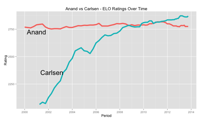
Let's say we want to look, year by year, how the two GMs have fared against each other. R has this great package called "plyr" which is tailor made for these kinds of "Split-Apply-Combine" type analyses. We are splitting the data by year, and combining based on win-loss, and plotting the tallies. The plotting package ggplot plays well with the output of plyr.

Once we do the plotting, we get a sense of what has been happening. In the early 2000s, Anand had a much higher share of wins. Overall the number of draws has gone up over the years. But Carlsen has had the upper hand the last year or two. (Of course, the number of games is too small, and we should be careful about "inferring" when the data is this tiny.) That said, we could make a strong the case that Carlsen has the momentum going for him.

4. Choice of Openings

Finally, we know that both GMs are holed up somewhere with their team of seconds and coaches, preparing. What do these experts prepare? A good majority of the times they are preparing opening surprises to spring on their opponents. They are studying each others' games looking for weaknesses. By looking at how their choice of openings helped them in the past, we can make a broad guess about what they might go.

R allows us to slice the data by their choice of openings, and we can see how they fared.

So we can expect that Anand will favor the openings that have more "green" (wins) for him, while Carlsen will try to play the openings that have been "red" (losses) for Anand.

By this logic, we can expect Anand to opt for the Queen's Gambit Declined-semi-slav(D47), the Ruy Lopez, closed (C96)  or the Sicilian closed (B23). Magnus will be trying to steer the game towards the English (A20) or the Benko (A58) which are slightly more unorthodox, but have served him well against Anand. The expansions behind the ECO list can be found here.

Of course, there will always be surprises. (This is where it all gets game-theoretical. If only it were this easy to predict...) And that's why we should watch what unfolds this November.

The R code used can be found here.

Ram

Using R to visualize Karpov-vs-Kasparov Lifetime winner-take-all tally

The Karpov vs. Kasparov rivalry holds a special place in the chess world.

The idea behind this analysis is simple. If we take their lifetime games, plot the wins, what would it look like? We introduce one twist -- we'll be plotting the "winner-take-all" tallies, meaning that for every year, every five years, and every decade, we declare one person to be the 'winner'.

First, a note of caution: "Winner-take-all" type analyses lose a lot of information due to the roll-up. Whether a GM wins by 1 game, or a dozen games in a given year, he still gets only one "win".

At the outset, I must mention that this is NOT a chess exercise. I am ignoring the colors (whether each player had White or Black pieces) and even more egregious, I don't differentiate between standard and rapid games, or exhibition games. Time controls are ignored, as are openings.

This is a visualization exercise, and the idea is to see how it all looks when plotted.

I scraped the data from chessgames.com - where they have 201 games that the two have played. (I cleaned up the data and the csv file is available in github for anyone who wants to do their own analysis.) I use plyr to aggregate the data, and ggplot for the visualization. I wanted to try out this "pianogram" type visualization, where each plot looks like piano-keys.

Let's get the basics out of the way:

201 games - 138 draws,  37 wins for Kasparov, 26 for Karpov

Overall, Kasparov pretty much dominated Karpov. But how are these wins and losses spread across time? The two played for a little over 30 years.

The Winner-Take-All Method
In any given time period, say 1990, there can be 4 possible outcomes:
No games played, Equal number of wins, Karpov won, or Kasparov won. (If both players had the exact same number of wins in a given time period, we label that a Draw.)

Thanks to the 'plyr' package and ggplot, we can calculate the by-year, "5-year Winner" for each half-decade, and also the decade-wise winners by writing one function, and calling it with ddply.


So here's what the Yearly-Winner-Take-All looks like:

Let's plot the half-decade and decade plots. Again, note that only one GM is declared the winner for the entire decade, no matter what the difference in the scores are.

Now, we can put it all together, in one graph.

As a very quick summary, we can see that Karpov started out strong, the entire 80's was a draw, and then Kasparov took over.

The complete R code to reproduce this analysis is available in this gist, along with the data-file in CSV file.