R - Defining Your Own Color schemes for HeatMaps

This post is intended at those who are beginners at R, and is inspired by a small post in Martin's bioblog.

First, we plot a "correlation heatmap" using the same logic that Martin uses. In our example, let's use the Movies dataset that comes with ggplot2.

We take the 6 genre columns, and we can compute the correlation matrix for those 6 columns.
Here's what the matrix looks like:

> cor(movieGenres) # 6x6 cor matrix
                  Action   Animation      Comedy        Drama
Action       1.000000000 -0.05443315 -0.08288728  0.007760094
Animation   -0.054433153  1.00000000  0.17967294 -0.179155441
Comedy      -0.082887284  0.17967294  1.00000000 -0.255784957
Drama        0.007760094 -0.17915544 -0.25578496  1.000000000
Documentary -0.069487718 -0.05204238 -0.14083580 -0.173443622
Romance     -0.023355368 -0.06637362  0.10986485  0.103545195
            Documentary     Romance
Action      -0.06948772 -0.02335537
Animation   -0.05204238 -0.06637362
Comedy      -0.14083580  0.10986485
Drama       -0.17344362  0.10354520
Documentary  1.00000000 -0.07157792
Romance     -0.07157792  1.00000000

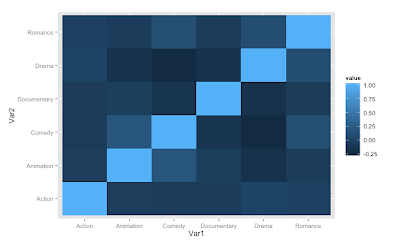
When we plot with the default colors we get:

It is difficult to see the details in the tiles. Now, if you want to better control the colors, you can use the handy colorRampPalette() function and combine that with scale_fill_gradient2.
Let's say that we want "red" colors for negative correlations and "green" for positives.
(We can gray out the 1 along the diagonal.)

Doing this produces:

If there are values close to 1 or to -1, those will pop out visually. Values close to 0 are a lot more muted.

Hope that helps someone.

References: Using R: Correlation Heatmap with ggplot2

R - Simple Recursive XML Parsing

This is intended for those who are starting out in R and interested in parsing an XML document recursively. It uses DT Lang's XML package.

If you want to just read certain types of nodes, then XPATH is great. This document by DT Lang is perfect for that.

However, if you want to read the whole document, then you have to recursively visit every node. Here's the way I ended up doing it. The generic function visitNode could be useful if you are just starting out reading XML in R.

The full code, along with a sample XML file to test it is here.

Simulating Allele Counts in a population using R

This post is inspired by the Week 7 lectures of the Coursera course "Introduction to Genetics and Evolution" (I highly recommend this course for anyone interested in genetics, BTW.) Professor Noor uses a Univ Washington software called AlleleA1 for trying out scenarios.

We can just as well use R to get an intuitive feel for how Alleles and Genotypes propagate or die out in populations.

Basic Scenario

There are N individuals in an isolated island. Say, we are interested in two specific Alleles (Big "A", or small "a"). This in turn means that they can have 3 types of genotypes: AA, Aa or aa. The individuals mate in pairs, and produce two offspring and die out. (Thus the total population remains the same generation after generation.)
The genotype of the offspring depends on those of the parents. A 'gamete' has only one parental allele, depending on what the parent's genotype was. AA type parent can only product gamete type A, aa parent can only produce gamete type a, but Aa can produce either type of gamete.

A Punnett square of parents gametes to offspring's genotypes. 

  | A  | a

 ---------------- 

A | AA | Aa 

a | Aa | aa 

With these simple rules, we can use R Simulation scripts to observe what happens to the Allele Frequencies over generations. (The goal here is to learn to use R for Monte Carlo simulations.)

Writing the R Script from scratch

 I toyed around with the idea of using character strings for the genotypes and the alleles. But then I realized that are only three types and I could just as easily represent them with the numbers 1, 2, 3 as a simple R vector.


With that done, we can write very simple functions for the procreation process.
With these useful functions, we can take one generation and produce another, 2 offspring for each set of 2 parents.
Putting it all together to generate multiple trials:

We also need to compute the Allele counts for each generation, and for plotting I use ggplot.



Using this simple Monte Carlo "toy" we can develop quite a bit of intuition.



For small starting populations, either the big A or the small a allele takes over the entire population fairly quickly. Given large enough number of generations, invariably one of the alleles gets wiped out.














As one example, we can see that even a small increase in the probability of Allele A to be 0.53 (up from 0.5) makes it take over quite dramatically.

Conversely, setting it to any value under 0.5 means that the Big A allele gets wiped out of the entire population.

The entire R script can be found here. You can download the code and try playing with various starting scenarios, changing the starting population counts, generations and probabilities.


References:

1. Coursera.org (Introduction to Genetics and Evolution by Md. Noor, Week 7 lectures) 
2. AlleleA1 software at Univ Washington